This is the second post in a series about spreadsheets, called Spreadsheets 101. Click if you missed the first post, Spreadsheets are Powerful. Here’s How.
Spreadsheets are powerful for an important reason: formulas. But if that feels like a scary word, let me reassure you. We’re not talking about the formula for finding compound interest (unless that’s what you need for your spreadsheet). In spreadsheet-speak, formulas are simple math sentences, using operations like addition and multiplication. They also employ the names of cells.
Cell, What’s Your Name?
First, remember that a cell in a spreadsheet is one of those little boxes in a spreadsheet. The best way to consider a cell is to think about it in terms of a column and row. The columns are identified by letters and the rows are numbered. So a cell’s name is identified by its letter (column) and number (row).
Take a look at the spreadsheet below. There are two cells with $300. What are their names?
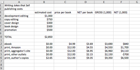
Did you guess B6 and B7? (It’s a little tough to see the numbers, but you can count from the top to the bottom.) If so, you’re right on target. Feel free to identify some additional cells, if you need a little more practice. Remember, these cell names are going to play a role in the formulas. So it’s important to be able to identify them correctly.
Symbolism
For the most part, you’ll probably use really simple formulas — finding the total of a set of numbers, finding the difference between two numbers, multiplying a value by another value. When you get into more complicated formulas, you may need to pay attention to the Order of Operations (PEMDAS). This is where parentheses can really come in handy. (We’ll focus on simple formulas in this post, leaving the more complex ones for another time.)
But first, you’ve got to know a little bit of shorthand. Because your computer does not have the same keyboard as a calculator, you’ll use ordinary keyboard symbols for a few of the math symbols. Take a look.
+ Addition
– Subtraction
* Multiplication
/ Division
^ Exponents
= A formula is coming!
Notice that the symbol for multiplication is not an “x.” This is because “x” means the letter x. (It can’t mean two things at once.)
The equals sign (=) tells the spreadsheet that a formula is coming. Otherwise, it would simply output the formula — and not the resulting value, after the formula is applied — in the cell. For that reason, each formula follows this pattern:
=(formula)
The word formula is the formula itself.
Now technically, you don’t need the parentheses around the formula, but I find it useful to use them. That’s because they’re necessary with all special formulas. Either way, you must have the equals sign.
Writing the Formula
Before writing the formula, think about what it is that you want to accomplish. In the spreadsheet above, the estimated costs and revenues from self-publishing a book are tabulated. In cell D16, the net for each printed authors copy is $9.35. That value was found using a formula.
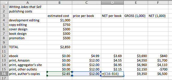
You can see this formula in the spreadsheet above: =(C16-B16). In other words, the net for each author’s copy is the price per book minus the estimated cost of producing the book. The price per book is in cell C16 and the estimated cost of one author copy is in cell B16. So the formula is =(C16-B16). Notice there are no spaces between any characters in the formula.
What about the net per ebook (cell D12)? The price of an ebook is quite a bit lower than a printed book, and there is no estimated cost. The net per ebook is found by multiplying the cost of the book by the royalty rate, which is usually a percentage. (Remember, you’ll need to convert the percentage to a decimal before you can multiply. Do that by moving the decimal place two places to the left.)
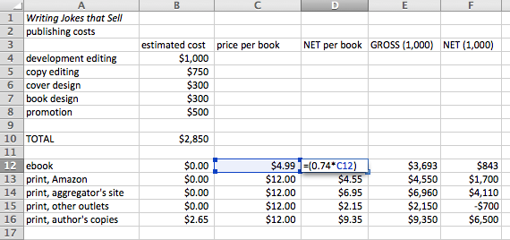
As you can see above, the formula used to find the net per ebook is =(0.74*C12), which means 74% of the value in C12. Notice that if you want to change the book price — to see how your numbers shake out with a lower or higher price — the net per book will automatically change. That’s because the formula pulls in whatever value you have in C12.
Special Formulas
There’s one more thing to consider: special formulas. If you find that you’re totaling long lists of values, you can use the SUM formula and select the values you want to total. Take a look at the example below.
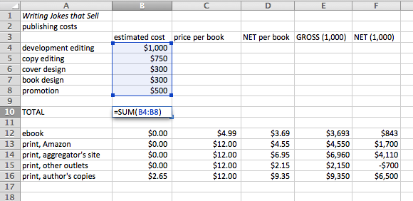
Cell B10 is the total of all publishing costs. In other words, you want to add all of the costs together. The formula =SUM(B4:B8) simply means this: Add all of the values in the cells from B4 through B8. In this case the colon means all of the values in the cells B4 through B8.
There is another way you can write this formula: =(B4+B5+B6+B7+B8). And if you want to do that, go for it. You’ll get the exact same answer. Of course the SUM formula is a simplified version of that same process.
And there are lots and lots of other special formulas. You can find these by nosing around in your spreadsheet program. These programs typically include a master list of special formulas. A Google search can unearth others.
So there you have it, a quick overview of using formulas in spreadsheets. This can be a lot more complex, depending on what you are doing. The key to remember is that a formula must appear between parentheses and after an equal sign. So play around with it. Don’t be afraid, you won’t break the program. If you find that you have some errors, stop by later to read my post on troubleshooting.
What special formulas have you found useful in spreadsheets? Do you have some advice to share or questions you need answers for? Talk to me in the comments section! And don’t forget to read my post about troubleshooting spreadsheets.
